Course Overview
This course introduces the fundamental ideas behind differential calculus, including topics such as limits, differentiation and the various rules that come with limits and differentiation.
As you progress through this course, you will find links to related topics in other courses (such as algebra). This interconnected structure is designed to help you quickly revisit prerequisite ideas without breaking your workflow.
Limits
We must begin with a discussion of what a limit is, why we care about it, and examples of when it is useful.
Suppose we have a funcion, say \(f(x) = x^2+1\), we might wonder what is the behavior of that function around a specific value of \(x\), for example \(x = 1\). We will make a table of values around that point to demonstrate the point.
| \(x\) | \(f(x)\) |
|---|---|
| 0.91 | 1.8281 |
| 0.92 | 1.8464 |
| 0.93 | 1.8649 |
| 0.94 | 1.8836 |
| 0.95 | 1.9025 |
| 0.96 | 1.9216 |
| 0.97 | 1.9409 |
| 0.98 | 1.9604 |
| 0.99 | 1.9801 |
| 1 | 2 |
| 1.01 | 2.0201 |
| 1.02 | 2.0404 |
| 1.03 | 2.0609 |
| 1.04 | 2.0816 |
| 1.05 | 2.1025 |
| 1.06 | 2.1236 |
| 1.07 | 2.1449 |
| 1.08 | 2.1664 |
| 1.09 | 2.1881 |
| 1.1 | 2.21 |
| 1.11 | 2.2321 |
Limits happen to be an extremely important tool in mathematics, and thankfully they are also quite easy to understand. One reason limits are so useful, is that we can determine if a function is continuous at a point, simply by taking the limit at that point. In the example above, we know that the function \(f(x) = x^2+1\) is continuous at \(x=1\) because the limit exists and is finite at that point. As we will see throughout the course, knowing that a function is continuous within an interval is extremely useful, as we will have a number of results that can take advantage of continuous functions. Another reason limits are useful, a fact that will be used over and over again in this course, is that limits allow us to understand the instantaneous rates of change in a function, something that Newton needed to understand mechanics, and as we will see, something that is used in many branches of the sciences now.
If you want the fast version, below is a short video introducing limits.
The Squeeze Theorem
Description of the squeeze theorem!
More to come!
Introduction to derivatives
Coming Soon
If you want the fast version, below is a short video introducing indeterminate products.
The Power Rule
Recall the definition of a derivative, \(f'(x) = \lim \limits_{h \rightarrow 0} \frac{f(x+h)-f(x)}{h}\). We are often interested in finding the derivatives of polynomial functions, that is functions \(P(x)\) where \(P(x) = a_0x^n + a_1x^{n-1} + ... + a_{n-1}x+a_n, n \in \{1,2,3,...,\}\), where \(a_0, a_1, ..., a_n\) are constants, and for the purposes of our discussion for now we will assume they are real numbers. So if our function \(f(x)\) is a polynomial function, then by the rules of limits, we may find the separate derivatives of each term of the polynomial and sum them together to find the complete derivative of the entire function. That is we can find the derivative of \(a_0x^n\) first, then find the derivative of \(a_1x^{n-1}\) and so on, and then add them all together to find the derivative. This works because the derivative is simply a limit, and limits of functions obey the rule that the limit of a sum is the same as the sum of the limits of those functions (provided the number of functions is finite, which is true of polynomials once we fix \(n\)). So, in general, we will be interested in finding the derivative of \(a_0x^n\), and for simplicity, we will begin by assuming \(a_0 =1\) for now (you should be able to verify later that even if the constant is not 1, it is very simple to deal with in the derivative in the sense that you can simply take the derivative of the function and then multiply it by the constant). Finally, since it will be useful for the discussion that follows if we include a description of the binomial theorem.
We will note that $$(x+h)^2 = x^2+2xh+h^2$$ if we multiply out the terms. Now if we multiply that by another \((x+h)\) so that we can get $$(x+h)^3 = (x^2+2xh+h^2)(x+h) = x^3+2x^2h+xh^2 + x^2h+2xh^2+h^3 = x^3+3x^2h+3xh^2+h^3.$$ Just for fun, lets go another step further, and then I will discuss the binomial theorem in full. $$(x+h)^4 = (x^3+3x^2h+3xh^2+h^3)(x+h) = x^4+3x^3h+3x^2h^2+xh^3+x^3h+3x^2h^2+3xh^3+h^4 = x^4+4x^3h+6x^2h^2+4xh^3+h^4.$$ We should take note of a few things that are happening as we increase the \(n\) in \((x+h)^n\). First if we look at the coeficient of the second term (with the terms ordered from the highest power of \(x\) to the lowest power), it is clear that this coeficient increases exactly linearly in \(n\), for example when \(n = 2\) the coeficient is \(2\), as we get the second term being \(2xh\), or when \(n = 3\) the coefficient is \(3\) for \(3x^2h\), similarly for \(n = 4\). Next, notice when ordered this way, the coefficients of the first and last term are always 1. What about the coefficients in between? This is a bit more challenging to show since we only went up to \(n = 4\), but you can verify if you wish by going to higher order that these coefficients show a particular pattern as well, and this is where the binomial theorem comes from. The binomial theorem states the following: $$(x+h)^n = x^n + nx^{n-1}h+\frac{n(n-1)}{2}x^{n-2}h^2 + ... + \binom{n}{k}x^{n-k}h^k+..>+nxh^{n-1}+h^n,$$ where \(\binom{n}{k} = \frac{n(n-1)\cdot \cdot \cdot (n-k+1)}{k!}\). Now that we have the binomial theorem, we are ready to see the key result. Notice that in the definition of the derivative that the \(x^n\) term will go away because we have, $$\lim \limits_{h \rightarrow 0}\frac{(x+h)^n - x^n}{h}$$, so the \(x^n\) term gets subtracted off, leaving only the terms with power of \(n-1\) or lower. The next term, based on the binomial theorem, will always have \(nx^{n-1}h\), and all of the following terms have powers of \(h\) that are 2 or higher. So when we divide through by \(h\) (from the definition of the derivative), we will get a leading term that looks like $$nx^{n-1}$$ and the remaining terms will all have \(h\) in them. It is easy to see, from the definition of the derivative (namely the \(\lim \limits_{h \rightarrow 0}\) part), that those terms will all go to zero in the limit (since all those remaining terms are multiplied by \(h\)), and the only thing that remains is $$nx^{n-1}$$. Thus, the derivative of \(x^n\) for any positive integer power \(n\), is \(nx^{n-1}\). This result is called the "power rule" for obvious reasons. This result is naturally very useful, since we often deal with polynomial functions, and additionally, there is a whole pretty large class of functions that can be represented by a Taylor series representation, which is an infinite series expansion of the function in terms of polynomials (note that Taylor series expansions cannot represent every function, but it can represent a large class of useful functions).
Now that we have the useful result, we should work on examples putting it to use. First I will start off simple, I want to find the derivative of \(f(x) = x^2\). According to the power rule the derivative (with \(n = 2\)) should be \(f'(x) = 2x\). We can verify this is correct by substituting directly into the limit, $$\lim \limits_{h \rightarrow 0} \frac{x^2 + 2xh + h^2 - x^2}{h} = \lim \limits_{h \rightarrow 0} \frac{2xh + h^2}{h} = \lim \limits_{h \rightarrow 0} 2x + h = 2x$$, which gives us the same answer as the power rule. You should challenge yourself and verify that the derivative of \(f(x) = x^3\), is \(f'(x) = 3x^2\) as shown by both the power rule and the limit definition of the derivative.
More to come!
Sum Rule For Derivatives
Now I want to do some examples of more complicated polynomials (the polynomial above only had a single term in it). For example, we will find the derivative of \(f(x) = 3x^3+2x\). But to do this we will need a couple of new rules, first is the sum rule of derivatives. Notice that we can think of this function as the sum of two functions \(f(x) = g(x) + k(x)\) where \(g(x) = 3x^3\) and \(k(x) = 2x\). This is a good time to show two important rules that arise in the limit definition of the derivative. The first one, is that any function that can be written \(f(x) = g(x) + k(x)\) has a derivative that can be written \(f'(x) = g'(x) + k'(x)\). To see this, start with the limit definition, $$\lim \limits_{h \rightarrow 0} \frac{f(x+h) - f(x)}{h} = \lim \limits_{h \rightarrow 0} \frac{g(x+h) - g(x)+ k(x+h) - k(x)}{h} = \lim \limits_{h \rightarrow 0} \frac{g(x+h) - g(x)}{h} + \frac{k(x+h) - k(x)}{h}$$ and by the rules of limits this means that $$\lim \limits_{h \rightarrow 0} \frac{g(x+h) - g(x)}{h} + \frac{k(x+h) - k(x)}{h} = \lim \limits_{h \rightarrow 0} \frac{g(x+h) - g(x)}{h}+ \lim \limits_{h \rightarrow 0} \frac{k(x+h) - k(x)}{h},$$ which by definition is \(g'(x) +k'(x)\). The second fact we need is that the derivative a function multiplied by a constant is the same as the constant multiplied by the derivative of that function.
Now we can move on to the constant multiple rule.
The Constant Multiple Rule
Suppose I have a function with a constant multiple in it (polynomials often have constants multiplying different powers of the independent variable for example). I will represent it as \(g(x) = cf(x)\) where \(c\) is the constant. Then, by the limit definition of the derivative, $$\frac{dg}{dx} = \lim \limits_{h \rightarrow 0} \frac{g(x+h)-g(x)}{h}.$$ Now note that we said \(g(x) = cf(x)\), so, $$\frac{dg}{dx} = \lim \limits_{h \rightarrow 0} \frac{cf(x+h)-cf(x)}{h} = \lim \limits_{h \rightarrow 0} c\frac{f(x+h)-f(x)}{h} = c\lim \limits_{h \rightarrow 0} \frac{f(x+h)-f(x)}{h},$$ where the last equal sign arises from the general rules for limits. Notice the simple rule here that arises, if I have a constant multiplying a function, then the derivative is just the constant times the derivative of the function. An amazingly simple rule!
Now we are ready to take the derivative of the polynomials, by combining the power rule, the sum rule and the constant multiple rule. To remind you of the example, suppose \(f(x) = 3x^3+2x\). By the sum rule, we can separate this into two functions, with \(g(x) = 3x^3, k(x) = 2x\), take their derivatives and add them together. That is \(f'(x) = g'(x)+k'(x)\). So we will first find \(g'(x)\). Now we can use the constant multiple rule, if we let \(l(x) = x^3,\) then \(g(x) = 3l(x)\), and thus \(g'(x) = 3l'(x) = 3(3)x^2 = 9x^2\), where we have applied the power rule in the middle step. Similarly, let \(m(x) = x\), then, \(k(x) = 2m(x)\), and since \(m'(x) = 1\) by the power rule, we have \(k'(x) = 2\).
I will make a final note here of warning, you will notice how powerful each of these rules are, especially when combined, as they make the computation of the derivative much easier than having to go back and use the limit definition of the derivative every time. This is great for computation, however, it allows people to forget entirely where the rules came from. My suggestion is that every time you use these rules, try and make sure you remember that all of the rules are inherited from limits and the limit definition of the derivative. As it turns out, limits are the most important part of calculus, and yet few people remember them after a calculus class!
Derivative of the natural log
Description of the the derivative for the natural log
More to come!
Derivatives of sinusoidal functions
Description of the the derivative for sinusoidal functions
More to come!
The Product Rule
Suppose now that I have a function that can be written as the product of two functions, that is, \(f(x) = g(x)k(x)\). Now if I want to find the derivative of this function \(f'(x)\), by the limit definition of the derivative I have, $$f'(x) = \lim \limits_{h \rightarrow 0}\frac{f(x+h)-f(x)}{h} = \lim \limits_{h \rightarrow 0}\frac{g(x+h)k(x+h) - g(x)k(x)}{h}.$$ Now we will use a common "trick" in mathematics, which is a clever addition by \(0\), so we will add and subtract the following \(g(x)k(x+h)\) (since we are adding the term and subtracting it, that works out to the same thing as adding by \(0\)), and we get, $$f'(x) = \lim \limits_{h \rightarrow 0}\frac{g(x+h)k(x+h)-g(x)k(x+h)+g(x)k(x+h) - g(x)k(x)}{h}.$$ Now we can reorganize, and use the rules of limits, namely that \(\lim \limits_{x \rightarrow a}g(x)+k(x) = \lim \limits_{x \rightarrow a}g(x) + \lim \limits_{x\rightarrow a}k(x)\), we find, $$f'(x) = \lim \limits_{h \rightarrow 0} k(x+h)\frac{[g(x+h)-g(x)]}{h} + \lim \limits_{h \rightarrow 0}g(x) \frac{[k(x+h)-k(x)]}{h},$$ and using another rule of limits (namely \(\lim \limits_{x \rightarrow a}g(x)k(x) = \Big(\lim \limits_{x \rightarrow a} g(x)\Big)\Big(\lim \limits_{x \rightarrow a} k(x) \Big)\)), $$f'(x) = \Big(\lim \limits_{h \rightarrow 0}k(x+h)\Big)\Big(\lim \limits_{h \rightarrow 0}\frac{[g(x+h)-g(x)]}{h}\Big) + \Big(\lim \limits_{h \rightarrow 0}g(x)\Big)\Big(\lim \limits_{h \rightarrow 0}\frac{[k(x+h)-k(x)]}{h}\Big).$$ Now note that by our assumptions \(k(x)\) will be continuous at \(x\) (otherwise this is not differentiable to begin with, so \(\lim \limits_{h \rightarrow 0}k(x+h) = k(x)\) and since there is no \(h\) at all in \(g(x)\), \(\lim \limits_{h \rightarrow 0}g(x) = g(x)\), this leaves us with, $$f'(x) = k(x)g'(x)+g(x)k'(x).$$
Now we should get some examples of actually using the product rule to our advantage. For example, suppose we have the function \(f(x) = \ln(x)x^2\). Let \(g(x) = \ln(x), k(x) = x^2\) We know from the natural logarithmic derivative rule, that \(g'(x) = \frac{1}{x}\) and from the power rule, \(k'(x) = 2x\). So from the product rule the derivative is, $$f'(x) = g'(x)k(x)+k'(x)g(x) = \frac{1}{x}(x^2)+(2x)\ln(x) = x+2x\ln(x).$$
For another example, consider \(f(x) = \ln(x)\cos(x).\) We will let \(g(x) = \ln(x), k(x) = \cos(x)\). Then, $$g'(x) = \frac{1}{x}, k'(x) = -sin(x),$$ where we found the derivative of \(k(x)\) using one of the sinusoidal function rules. Thus, applying the product rule we find that, $$f'(x) = g'(x)k(x)+k'(x)g(x) = \frac{1}{x}(\cos(x)) - \sin(x)\ln(x).$$
We should note that we have given the special case of when we have the product of two functions only. However, in general, we can find the derivatives of products with more than two functions by repeated application of the product rule. For instance, suppose we have a function \(f(x)\) which can be written as \(f(x) = g(x)k(x)l(x)\). Then note that \(f(x) = [g(x)k(x)]l(x).\) So this looks like the product of a product, we can apply the product rule twice. $$f'(x) = [g'(x)k(x) + k'(x)g(x)]l(x) + [g(x)k(x)]l'(x) = g'(x)k(x)l(x) + k'(x)g(x)l(x) + g(x)k(x)l'(x).$$ Notice that we applied the product rule to the object in the square brackets first to find the derivative of \(g(x)k(x)\) and then applied the product rule to the outer portion (or however you want to look at it). For example, suppose we have, \(f(x) = x^2\ln(x)\cos(x).\) Then the derivative is, $$f'(x) = g'(x)k(x)l(x) + k'(x)g(x)l(x) + g(x)k(x)l'(x) = (2x)\ln(x)\cos(x) + (\frac{1}{x})x^2\cos(x) + x^2\ln(x)(-\sin(x)) = (2x)\ln(x)\cos(x)+x\cos(x)-x^2\ln(x)\sin(x).$$
The Quotient Rule
Description of the quotient rule!
More to come!
The Chain Rule
It will benefit us to remind ourselves what it means to be differentiable here. For a function to be differentiable at a point, the limit in the limit definition of the derivative must exist and be finite. So for the remainder (and this is an important point, since what follows will not work if there is any point in the domain of interest where the function is not differentiable) of this section we will assume all functions are differentiable across the domains of interest (yes, there will be MULTIPLE domains). Suppose we have the composition of two functions, say \(f\) and \(g\), so that we have \(f(g(x))\). We may be interested in finding the derivative of this composition, we want to find \(f'(x)\). If we assume that \(g\) is differentiable with respect to \(x\) across the domain of \(x\) and that \(f\) is differentiable with respect to \(g(x)\) across the domain of \(g(x)\), then we can use a simple "trick" to find the derivative . Note that, by the limit definition of the derivative, $$\frac{d}{dx}f(g(x)) = \lim \limits_{\Delta x \rightarrow 0} \frac{\Delta f}{\Delta x},$$ note here we have slightly shifted notation for convenience, we can assume \(\Delta f = f(x+h)-f(x), \Delta x = (x+h)-x = h\). Then we will simply multiply by \(1\), noting that \(\frac{\Delta g}{\Delta g} = 1\) assuming \(\Delta g \neq 0\). Thus, $$\frac{d}{dx}f(g(x)) = \lim \limits_{\Delta x \rightarrow 0} \frac{\Delta f}{\Delta x}\frac{\Delta g}{\Delta g} = \lim \limits_{\Delta x \rightarrow 0} \frac{\Delta f}{\Delta g}\frac{\Delta g}{\Delta x}.$$ Now, using another rule we know about limits, namely that the limit of a multiplication is the same as the multiplication of the limits, we can rewrite this as, $$\frac{d}{dx}f(g(x)) = \Big(\lim \limits_{\Delta x \rightarrow 0} \frac{\Delta f}{\Delta g}\Big)\Big(\lim \limits_{\Delta x \rightarrow 0}\frac{\Delta g}{\Delta x}\Big).$$ The last part in our proof of the chain rule requires a bit of a conceptual explanation. Since we are assuming \(g(x)\) is differentiable with respect to \(x\), this means it must be continuous with respect to \(x\) (please do note that the converse is NOT true, a function that is continuous at a point is NOT necessarily differentiable at that point, and this will be a key distinction). Since \(g(x)\) is continuous then it MUST be true that \(\Delta g \rightarrow 0 \ \mbox{as,} \ \Delta x \rightarrow 0\). If this wasn't true then \(g(x)\) would have to be discontinuous because \(g(x)\) would have to take on a different value depending on which way \(x\) tended to \(0\). Phew, since we have now established (again we needed to assume differentiability!) that \(\Delta g \rightarrow 0 \ \mbox{as,} \ \Delta x \rightarrow 0\), we can replace in the relevant portion \(\Delta x\) with \(\Delta g\), thus, $$\frac{d}{dx}f(g(x)) = \Big(\lim \limits_{\Delta g \rightarrow 0} \frac{\Delta k}{\Delta g}\Big)\Big(\lim \limits_{\Delta x \rightarrow 0}\frac{\Delta g}{\Delta x}\Big).$$ This leaves us with the final result of the chain rule, which states that, $$\frac{d}{dx}f(g(x)) = f'(g(x))g'(x).$$ Now this result may actually be one of the most important results we have, often times functions can be represented quite easily as compositions of multiple functions, and we can have instances with repeated (nested) usage of the chain rule. The chain rule is even used in neural networks, which is what allows "back-propogation" a key detail that makes neural networks work well. Now we should give a couple of examples to demonstrate the usefulness of the chain rule.
Suppose I have the function \(k(x) = \sqrt{3x^3}\) and I want to find it's derivative. Clearly this function can be written with \(f(x) = \sqrt{x}, g(x) = 3x^3\), thus if we let \(k(x) = f(g(x))\), we can see that we have the composition of two functions. Using the chain rule, to find \(k'(x)\) we must find \(f'(g(x))\) and separately find \(g'(x)\) and multiply them together. To find \(f'(g(x))\) we will note again that \(g'(x) = 3x^3\), and note that \(f'(x) = \frac{1}{2}x^{\frac{-1}{2}} = \frac{1}{2}\frac{1}{\sqrt{x}}\), thus \(f'(g(x)) = frac{1}{2}\frac{1}{\sqrt{3x^3}}\) using the power rule, and note that \(g'(x) = 9x^2\) using the constant multiple rule and the power rule together. So finally, $$k'(x) = f'(g(x))g'(x) = \frac{1}{2}\frac{9x^2}{\sqrt{3x^3}}$$
Indeterminant Forms
In this section we will be rehashing limits. If you have forgotten about limits, I strongly suggest that you click here to remind yourself of how to perform them. It should be no surprise, from how this course has progressed thus far, that we will find ourselves interested with the behavior of functions as they approach certain values. However, we may run into an issue in certain places, for example, suppose we are interested in the following rational function, $$F(x) = \frac{x^2-1}{x-1},$$ and specifically we want to know the value of \(F(x)\) as \(x \rightarrow 0\), thus we should write this as $$\lim \limits_{x \rightarrow 1} F(x) = \lim \limits_{x \rightarrow 1} \frac{x^2-1}{x-1},$$ of course the problem is, that as we approach 1 from either the left or the right we end up with \(F(x) \rightarrow \frac{0}{0}\). The problem that we are running into here is that \(\frac{0}{0}\) is undefined. This is one example of what is called an indeterminant form, \(\frac{\pm \infty}{\pm \infty}\) is another example, and there are a number of other indeterminant forms as we will see through the examples below. I want to take a moment to note how appropriate the name is, these forms are indeterminate because as we will see in the following sections, we can't (necessarily) determine beforehand what the answer will be, for instance \(\frac{\infty}{\infty}\) could be 1 or it could be \(\infty\) or it could be any real number you can choose depending on the functions involved!
If you want the fast version, below is a short video introducing indeterminant forms.
So how do we handle this problem of indeterminate forms? Well, we can handle it algebraically in some cases, the example given above is an ideal candidate for this. Notice that we can factor the numerator since it is the difference of two perfect squares, which will allow us to make a cancellation (we must be very cautious with these types of cancellation because for instance in this case it is only valid if \(x\neq1\), but we get "away" with that here because we are taking limits, not setting it equal to 1), $$\frac{x^2-1}{x-1} = \frac{(x+1)(x-1)}{(x-1)} = x+1,$$ which is true, as noted above, for \(x \neq 1\). This is perfectly fine from a limit standpoint, we are only asking the behavior as \(x\) approaches 1. So if we take the limit here, $$\lim \limits_{x \rightarrow 1} x+1 = 2.$$
This is nice, but as you probably guessed from my comment above "in some cases" that this method is not overly general. Indeed, in many cases using this type of trick is impossible. So instead, we will ask for a more general method, which I will discuss below called l'Hospital's rule.
l'Hospital's rule
I will start by stating l'Hospital's rule and then we will begin discussing applications. Suppose we have two differentiable functions, \(f\) and \(g\), and furthermore that \(g \neq 0\) and \(f,g\) are both differentiable on some open interval \(I\) around \(a\) (though it may not contain \(a\) itself). Additionally suppose either, \(\lim \limits_{x \rightarrow a}f(x)=0\) and \(\lim \limits_{x \rightarrow a}g(x)=0\) or \(\lim \limits_{x \rightarrow a}f(x)=\pm \infty\) and \(\lim \limits_{x \rightarrow a}g(x)=\pm \infty\) (notice the ratio of these functions will be in common types of indeterminate forms), then $$\lim\limits_{x\rightarrow a}\frac{f(x)}{g(x)} = \lim\limits_{x\rightarrow a}\frac{f'(x)}{g'(x)},$$ so long as the limit of the right hand side exists. In other words, the limit of ratio of the functions is the same as the limit of the ratio of each functions derivative. We can continue using our example from the last section and verify that we get the same answer. Recall that click here from the power rule, if we let \(f(x) = x^2-1\), then $$f'(x) = 2x.$$ Similarly, using the power rule, since \(g(x) = x-1\) then \(g'(x) = 1\). Thus according to l'Hospital's rule, we have $$\lim \limits_{x \rightarrow 1} \frac{x^2-1}{x-1} = \lim \limits_{x \rightarrow 1} \frac{2x}{1} = 2,$$ which is identically what we found above! So now we should work on some examples which we can't simply manipulate algebraically, which shows the real power of l'Hospital's rule.
If you want the fast version, below is a short video introducing l'Hospital's rule.
Suppose we have the function \(K(x) = \frac{\mbox{cos}(x)}{x-\frac{\pi}{2}}\) and we want to find the limit of this function as \(x \rightarrow \frac{\pi}{2}\). Notice we will run into the \(\frac{0}{0}\) indeterminate form. Thus, recalling derivatives of sinusoidal functions and the power rule, if we let \(f(x) = \mbox{cos}(x), f'(x) = -\mbox{sin}(x)\) and \(g(x) = x-\frac{\pi}{2}, g'(x) = 1\). Now taking the limit, $$\lim\limits_{x \rightarrow \pi/2}\frac{\mbox{cos}(x)}{x-\frac{\pi}{2}} =\lim\limits_{x \rightarrow \pi/2} \frac{-\mbox{sin}(x)}{1} = -1.$$ Notice that there was no easy algebraic manipulation to get to this result, but straightforward application of l'Hospital's rule worked beautifully!
OK, but I mentioned there were other indeterminate forms, specifically I already mentioned \(\frac{\pm \infty}{\pm \infty}\), so we will take a look at some examples there. Suppose for example, that \(Q(x) = \frac{-3x^3-5x^2}{2x^3-1}\) and we wish to understand the behavior of this function as \(x \rightarrow \infty\) (this, by the way, is often a question asked in physics, what happens as I get "very far away" from whatever pheonomena I am observing?) Notice the problem we have, if I let \(f(x) = -3x^3-5x^2\) then as \(x \rightarrow \infty, f(x) \rightarrow -\infty\) and similarly, if I let \(g(x) = 2x^3-1\) as \(x \rightarrow \infty, g(x) \rightarrow \infty\). So I have the indeterminate form \(\frac{-\infty}{\infty}\) to be specific. According to l'Hopital's rule, $$\lim\limits_{x \rightarrow \infty}Q(x) = \lim\limits_{x \rightarrow \infty}\frac{-9x^2-10x}{6x^2},$$ after applying the power rule to both the numerator and the denominator. But this time notice that I have a problem, I still get the indeterminate form \(\frac{-\infty}{\infty}\), but notice that I am getting somewhere, as the power has been reduced in each of \(f,g\). So, the natural thing to do here is to apply l'Hospital's rule again, $$\lim\limits_{x \rightarrow \infty}Q(x) = \lim\limits_{x \rightarrow \infty}\frac{-18x-10}{12x},$$ but again we have the same problem, but we are much closer now. So apply the rule yet again, $$\lim\limits_{x \rightarrow \infty}Q(x) = \lim\limits_{x \rightarrow \infty}\frac{-18}{12},$$ now that is NICE!. We see that the limit is \(\frac{-18}{12}= \frac{-3}{2}\). We should take a look at another example to flesh out our understanding. For example, imagine the function \(r(x) = \frac{x^3}{x^2}\) and imagine that we want to find the behavior as \(x \rightarrow \infty\). Well, we should be able to immediately identify that this is of the form \(\frac{\infty}{\infty}\), so we will apply l'Hospital's rule: $$\lim\limits_{x \rightarrow \infty}r(x) = \lim\limits_{x \rightarrow \infty}\frac{3x^2}{2x},$$ but we can see that leavies us with an indeterminate form still, so applying again, $$\lim\limits_{x \rightarrow \infty}r(x) = \lim\limits_{x \rightarrow \infty}\frac{6x}{2},$$ but this gets us \(\frac{\infty}{2}\) which is NOT an indeterminate form, this is just \(\infty\). So we have found that \(\lim\limits_{x \rightarrow \infty}r(x) = \infty\). To link this to what I said in the indeterminate forms section, the past 2 examples show why these forms are called indeterminate, it is because in both cases we had something of the form \(\frac{\pm \infty}{\pm \infty}\), and for one of them it turned out that this led to \(\frac{-3}{2}\) and in the other case it led to \(\infty\)! We will check out other indeterminate forms in the next section.
Indeterminate Products
Coming Soon
If you want the fast version, below is a short video introducing indeterminate products.
The Extreme Value Theorem
Coming Soon
If you want the fast version, below is a short video introducing indeterminate products.
Directional Derivatives
Notice the level sets (contours) of the image of Mount Fuji. These represent the curves of constant elevevation (why not call that \(z(x,y)=c\), where \(c\) is the constant
elevation).
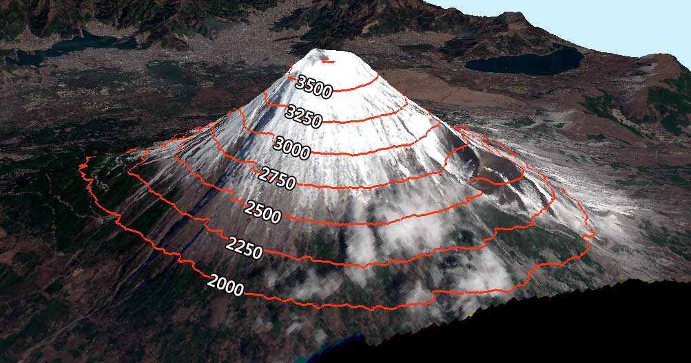 The partial derivative \(z_x\) represents the derivative (rate of change) along the \(x\) direction and \(z_y\) represents the derivative along the \(y\) direction.
But what if I want to know the rate of change along some other direction, such as at a \(45^o\) angle between \(x\) and \(y\)? This brings in the concept of the
directional derivative. Recall that at a single point \((x_0,y_0\) we define the partial derivative
$$z_x(x_0,y_0) = \lim \limits_{h \rightarrow 0} \frac{z(x_0+h,y_0)-z(x_0,y_0)}{h},$$
and
$$z_y(x_0,y_0) = \lim \limits_{h \rightarrow 0} \frac{z(x_0,y_0+h)-z(x_0,y_0)}{h},$$
where these represent the changes in the unit direction \(\mathbf{i}\) and \(\mathbf{j}\) respectively. If we now would like to know the rate of change along some unit vector
\(\mathbf{u} = \langle a,b \rangle \). In this case we need to recognize that we are "splitting" \(h\) along two directions, and they are being scaled by \(a\) and \(b\) along
those directions. That is, in the \(x,y\) plane, \(h^2 = (ah)^2+(bh^2)\) using Pythagorean theorem (thankfully we are working in a flat plane and this still applies!). This means
that \(x-x_0 = ah, y-y_0 = bh\). And so, since these represent the legs (with \(h\) as the hypoteneuse) we can define the directional derivative along this direction at
point \((x_0,y_0)\) as,
$$D_u z(x_0,y_0) = \lim \limits_{h \rightarrow 0}\frac{z(x_0+ah,y_0+bh)-z(x_0,y_0)}{h},$$
if the limit exists, naturally.
The partial derivative \(z_x\) represents the derivative (rate of change) along the \(x\) direction and \(z_y\) represents the derivative along the \(y\) direction.
But what if I want to know the rate of change along some other direction, such as at a \(45^o\) angle between \(x\) and \(y\)? This brings in the concept of the
directional derivative. Recall that at a single point \((x_0,y_0\) we define the partial derivative
$$z_x(x_0,y_0) = \lim \limits_{h \rightarrow 0} \frac{z(x_0+h,y_0)-z(x_0,y_0)}{h},$$
and
$$z_y(x_0,y_0) = \lim \limits_{h \rightarrow 0} \frac{z(x_0,y_0+h)-z(x_0,y_0)}{h},$$
where these represent the changes in the unit direction \(\mathbf{i}\) and \(\mathbf{j}\) respectively. If we now would like to know the rate of change along some unit vector
\(\mathbf{u} = \langle a,b \rangle \). In this case we need to recognize that we are "splitting" \(h\) along two directions, and they are being scaled by \(a\) and \(b\) along
those directions. That is, in the \(x,y\) plane, \(h^2 = (ah)^2+(bh^2)\) using Pythagorean theorem (thankfully we are working in a flat plane and this still applies!). This means
that \(x-x_0 = ah, y-y_0 = bh\). And so, since these represent the legs (with \(h\) as the hypoteneuse) we can define the directional derivative along this direction at
point \((x_0,y_0)\) as,
$$D_u z(x_0,y_0) = \lim \limits_{h \rightarrow 0}\frac{z(x_0+ah,y_0+bh)-z(x_0,y_0)}{h},$$
if the limit exists, naturally.
More to come!